Human perception of clusters in Gaussian-distributed fields of dots
Roanoke College
What is a cluster?
These slides available at: https://floruit.xyz/static/wic/Cate_CVCSN_2024.html
- Many studies of dot perception, including with regard to estimating number
- Nearly always “randomly distributed” (Poisson)
- Never Gaussian
 Allik & Tuulmets (1991)
 Anobile, Cicchini & Burr (2013)
 Im, Zhong & Halberda (2016)
Different stimulus distributions
Animations looping through all 180 patterns viewed by participants
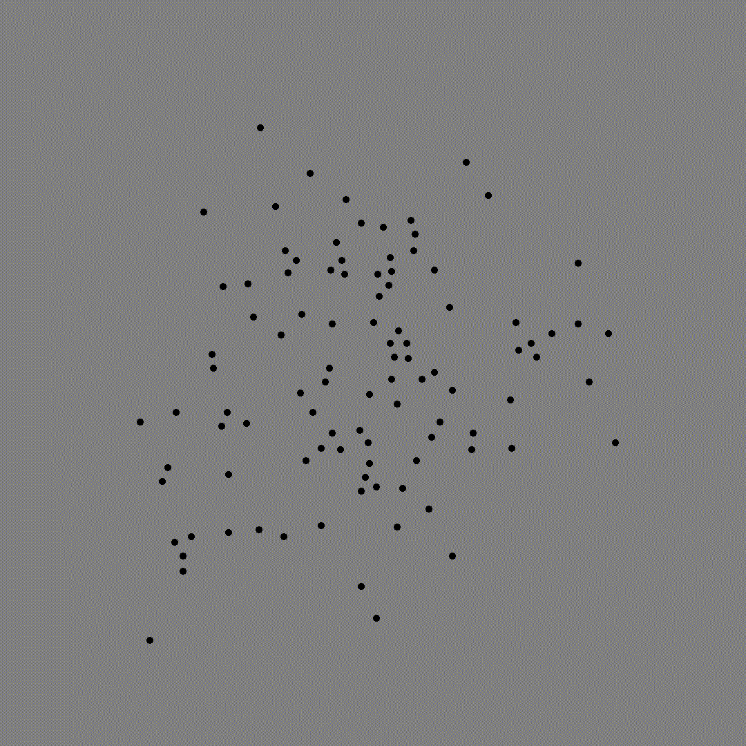
Gaussian, \(\sigma\) = 1.7
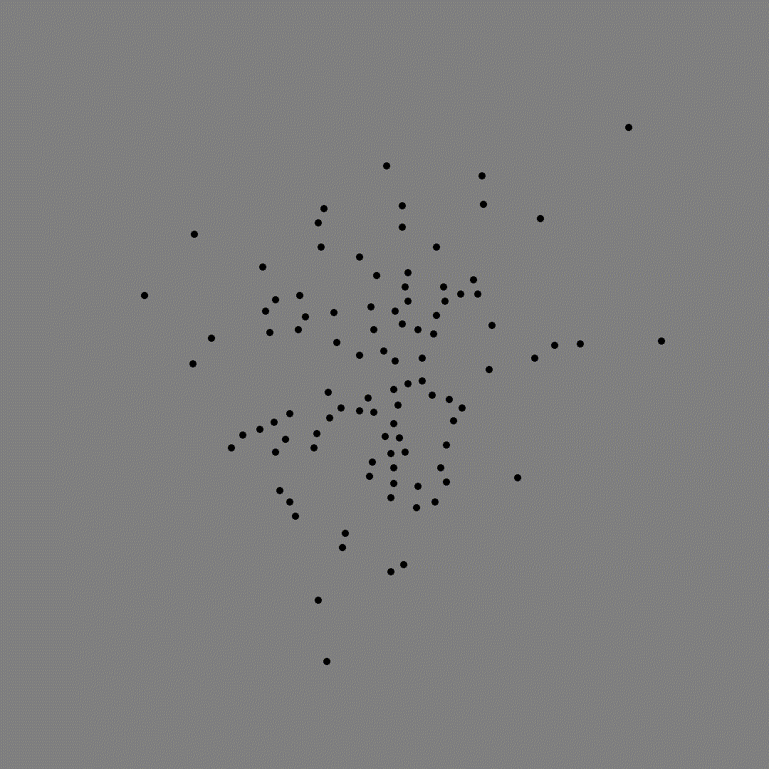
Gaussian, \(\sigma\) = 2.0
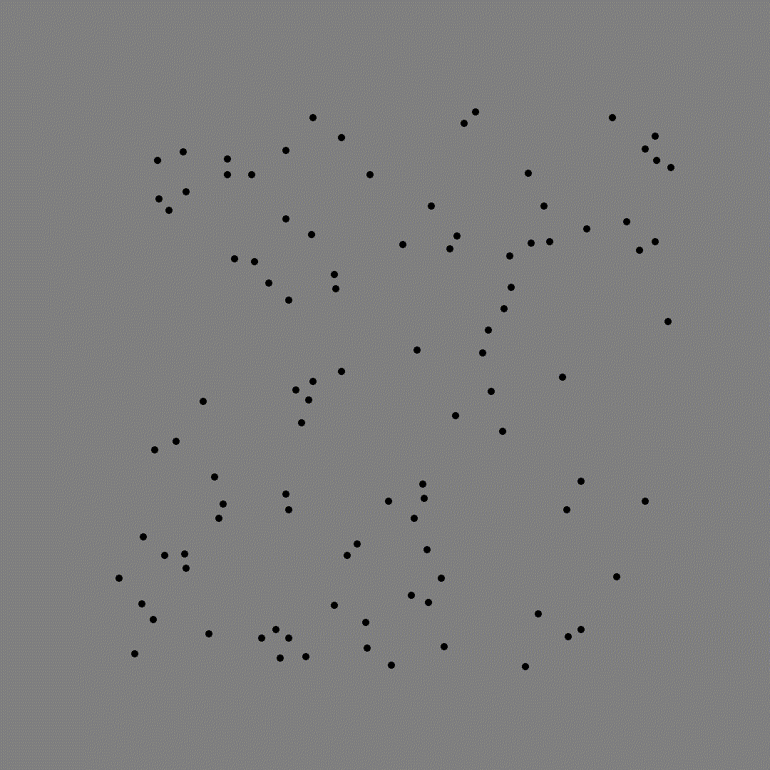
Poisson
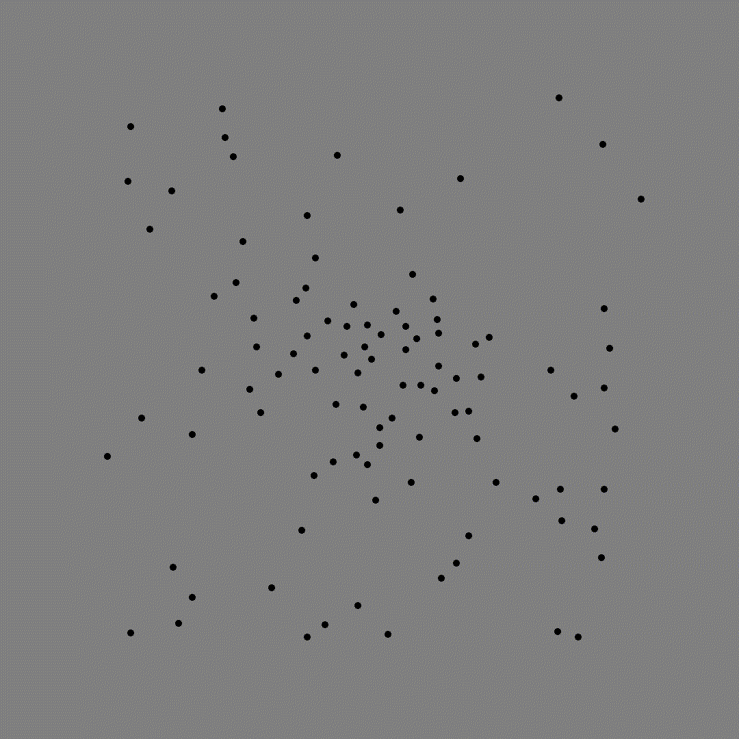
Gaussian, \(\sigma\) = 4.0, with Poisson “pedestal”
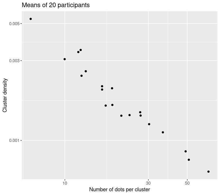
Measure density of selected clusters
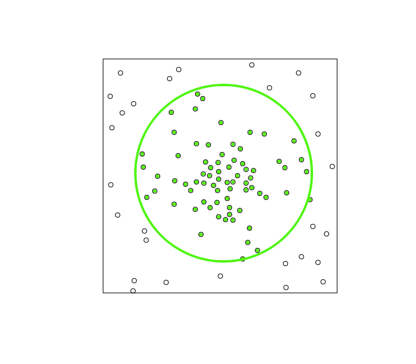
 Use convex hull to measure area of clusters

Simulated clusters from expanding rings


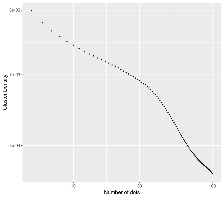
Baseline data for comparison
Assume that simplest cluster formation method is to select all dots within a given radius of display center
Recalculate cluster measurements for clusters of different numbers of dots: from 1 to 100 dots
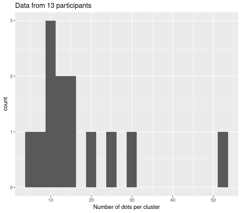
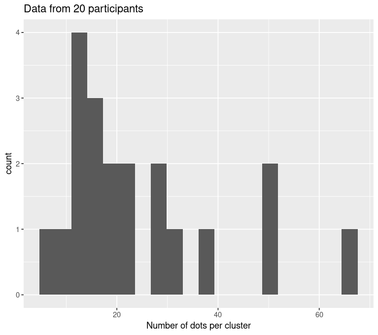
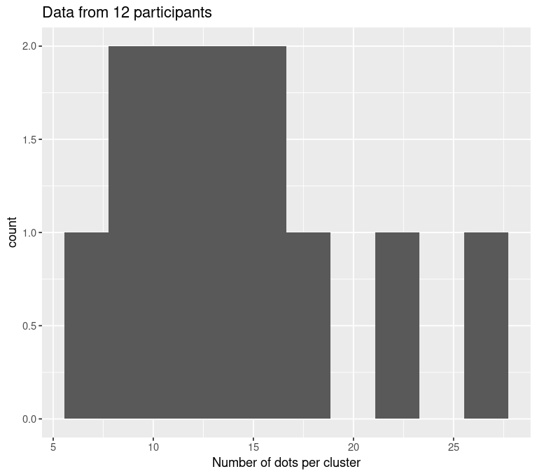
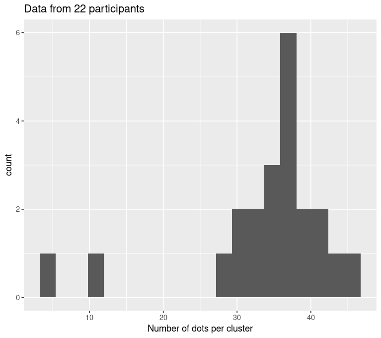
Different sized dot clusters chosen by participants
Gaussian, \(\sigma\) = 1.7
Gaussian, \(\sigma\) = 2.0
Poisson
Gaussian, \(\sigma\) = 4.0, with Poisson “pedestal”
Significance of the cluster densities chosen by participants


Linear mixed effects regression: Type II Wald \(\chi^2\) = 180.26, p << 0.001

Green ribbon = standard error of the mean for simulated baseline data (from 180 trials) \(y = f(x) = cluster\ density(number\ of\ dots)\)

Yellow dots = inflection points (\(y'' = 0\))
Purple dot = maximum of Gaussian curvature \(\kappa\) of baseline data curve \[ \kappa\left(x\right) = \frac{{\lvert}y''{\rvert}}{\left(1 + \left(y'\right)^2\right)^\frac{3}{2}} \]
Gaussian Distributed Dots, STD = 1.7
Linear mixed effects regression: Type II Wald \(\chi^2\) = 180.26, p << 0.001
Gaussian Distributed Dots, STD = 2.0

Linear mixed effects regression: Type II Wald \(\chi^2\) = 209.03, p << 0.001
Poisson distributed points

Linear mixed effects regression: Type II Wald \(\chi^2\) = 87.5, p << 0.001
Gaussian Distributed with Poisson “pedestal”


Linear mixed effects regression: Type II Wald \(\chi^2\) = 190.63, p << 0.001


Power Law Selection of Cluster Density
Straight lines on log-log axes indicate power functions:
\(f(x) = ax^k + b\)
Log-log slope = the exponent (\(k\)), intercept = slope (\(a\))
Stevens’ Power Law: intensity of perceptual phenomena follow power functions
- Different phenomena characterized by different exponents
Cluster density: negative slopes -> negative exponents
- Small quantities of dots form highly dense clusters with rapid reduction in density after a few tens of dots
- Then only very gradual reduction in density